In a break from the (til now) norm, I’m going to talk about a topic I adore: Chaos. I will try to make most of this post relatable for the layman.
What the hell is it?
In the sense of the dictionary, chaos is some occurrence that seems so unpredictable as to appear random. In the physics & mathematics world, we have a slightly more technical definition:
Chaos is the behavior of dynamics systems that are highly sensitive to initial conditions.
For the uninitiated, let’s start with some basic terms from that sentence:
- System – a series of connected parts that operate together to produce some measurable output. An electrical circuit, a mechanical device, a chemical process. These can all be modeled as systems.
- Dynamics – the study of the change of these systems over time. This is in comparison to statics, where the system is unchanging.
- Initial conditions – the starting point of the system. Think of ball in a bowl. It can begin in the bottom of the bowl, along the sides, or at the top.
- Highly sensitive – small changes in the initial conditions lead to large differences in the end result.
For a textbook version of non-chaotic systems, we can look to the archetypal Van Der Pol oscillator in two dimensions:
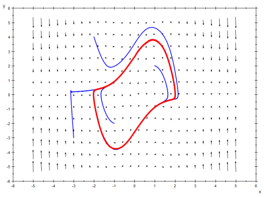
Phase Portrait of the Van Der Pol oscillator (source: Wikipedia.)
This oscillator is a model of an electronic circuit that has a cyclical output under certain conditions (check out wiki for the schematics). Even for those unfamiliar with dynamic systems and phase portraits, you can interpret the image above like this: the blue lines are the path of the system starting at some arbitrary point. Think of the graph as a topography with the arrows pointing downhill, and the system as a drop of rain that flows with gravity.
At some particular space on the phase portrait, the system is being “pushed” in some direction. For example, you can see that at the edges of the plot, it is being pushed towards the center in every position.
The red “pool” shape is an orbit that the system gets locked into, a pattern that keeps repeating itself. As you can see from the portrait, no matter where you start you end up in the pool orbit.
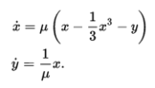
2D Van Der Pol Equations
For the geeks like me, I’ve attached the 2D variant of the Van Der Pol equations above. These (x-dot and y-dot) are the equations of the slopes (or gradient) in each direction, at a particular point on the phase portrait. μ is a constant value that changes the shape of the pool, and is ~1.5 for the plot above. Plug in a value of x or y on the portrait (say X=10, Y = 10), and you’ll see that the sum of those vectors gives you the direction and magnitude of the arrow at that point.
The Lorenz Butterfly
The go-to demonstration of nonlinear chaos is the Lorenz Strange Attractor, also known as the Lorenz Butterfly. Lorenz came across this system when he was studying atmospheric convection – the study of heat being passed through the air from the warm equator areas of Earth into the areas nearer the poles.
I’ve put together an animation in MATLAB to show two things:
- How awesome chaos in three dimensions is, and
- The sensitivity to initial conditions. The black point starts at (x, y, z) = (1, 1, 1), and the magenta point starts at (x, y, z) = (1.1, 1.1, 1.1).
Pay special attention at the beginning to where the two points start, how rapidly they start to veer apart, and where the tracks decide to switch sides of the butterfly. Also notice that there appear to be two attractors, points that the system hovers around, but never crash into, like the pool in the Van Der Pol oscillator.
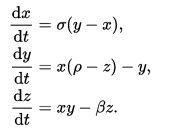
Ordinary Differential Equations for the The Lorenz Attractor
Since we’re in three dimensions, there’s an extra equation for the system. Naturally, the phase portrait would also be three dimensional, and tough to display. In these equations, dx/dt, dy/dt, and dz/dt are equivalent to x-dot in the oscillator. They determine the gradient in the phase portrait at a point (x, y, z). The fancy Greek letters (σ, ρ, β) are again constants like μ. In this case, (σ, ρ, β) = (28, 10, 8/3).
So, fun stuff! It always fascinates me how rather unassuming physical systems can lead to surprising dynamic studies. If you’re interested in this topic, I recommend Nonlinear Dynamics and Chaos by Strogatz.
